Example: Two phases model, extension followed by compression
This example shows how to build a model with 2 tectonic phases. For the example we consider a model with a first phase of orthogonal extension followed by a second phase of oblique compression. Following the same pattern, it is possible to have a first phase of compression followed by a second phase of extension. However, the example only covers a model with two tectonic phases. No API is currently available for more than two phases but it is theoretically possible.
Note
This example shows a case where the direction of extension and compression are different. In the case they are the same, it is not required to produce one options file per phase.
1. Create a domain
We define a 3D Domain \(\Omega = [0,600]\times[-250,0]\times[0,300]\) km3
\(\in \mathbb R^3\) discretized by a regular grid of 9x9x9 nodes.
import os
import numpy as np
import genepy as gp

# 3D domain
dimensions = 3
O = np.array([0,-250e3,0],    dtype=np.float64) # Origin
L = np.array([600e3,0,300e3], dtype=np.float64) # Length
n = np.array([9,9,9],         dtype=np.int32)   # Number of Q1 nodes i.e. elements + 1
# Create Domain class instance
Domain = gp.Domain(dimensions,O,L,n)
2. Velocity field
We define two velocity fields, one for the extension phase and one for the compression phase.
2.1. Extension phase
The extension velocity field is defined as a orthogonal extension of 1 cm.a-1 in the \(x\) direction.
u_params  = {"u_norm"        : 1.0 * cma2ms,     # norm of the velocity on boundary
             "variation_dir" : "x",              # direction in which velocity varies
             "velocity_type" : "extension",      # extension or compression (because norm > 0)
             "u_angle"       : np.deg2rad(90.0)  # angle of the velocity vector
            }
# Create linear velocity class instance
phase_1   = gp.VelocityLinear(Domain,**u_params)
2.2. Compression phase
The compression velocity field is defined as a 45 degrees compression of 3 cm.a-1 in the \(x\) direction.
u_params  = {"u_norm"        : 3.0 * cma2ms,     # norm of the velocity on boundary
             "variation_dir" : "x",              # direction in which velocity varies
             "velocity_type" : "compression",    # extension or compression (because norm > 0)
             "u_angle"       : np.deg2rad(45.0)  # angle of the velocity vector
            }
# Create linear velocity class instance
phase_2   = gp.VelocityLinear(Domain,**u_params)
2.3. Combine the two phases
First we define the time at which the tectonic phases change:
# time inversion parameters
Ma2s = (3600.0 * 24.0 * 365.0) * 1e6 # Million years to second conversion
t1   = 2.0 * Ma2s
t2   = 4.0 * Ma2s
breakpoints = np.array([ t1, t2 ],       dtype=np.float64) # breakpoints in time (where atan(t-t0)=0 )
slopes      = np.array([ 5e-13, 5e-13 ], dtype=np.float64) # slope s of h(t) = s(t-t0) for atan(h(t)) function
Then we combine the two velocity fields and evaluate the time-dependant velocity
using the VelocityInversion class
# create time dependant velocity inversion class instance
bc_inv = gp.VelocityInversion(Domain,phase_1,phase_2,breakpoints,slopes)

# Access the symbolic velocity function, its gradient and the orientation of the horizontal velocity at the boundary
u      = bc_inv.u                   # velocity function
grad_u = bc_inv.grad_u              # gradient of the velocity function
uL_1   = bc_inv.u_dir_horizontal[0] # orientation of the extension phase
uL_2   = bc_inv.u_dir_horizontal[1] # orientation of the compression phase
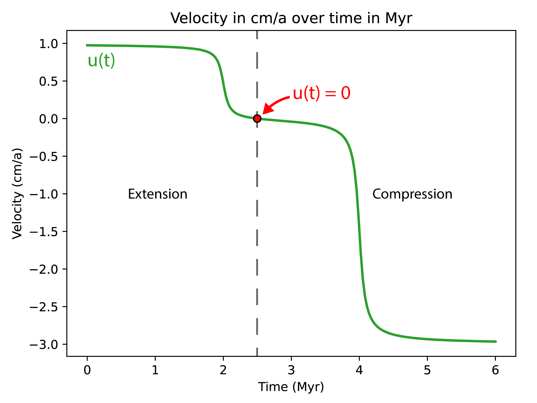
To help visualize the resulting time dependant velocity function a
plotting method using matplotlib is available:
# plot the 1D velocity profile over time
time_1d = np.linspace(0, 6, 201) * Ma2s # time array for plot
bc_inv.plot_1D_velocity(time_1d)
This function uses the norm of the velocity to plot the velocity profile over time.
The sign convention used is that the velocity is positive for extension and negative for compression.
In addition, if the velocity should pass through zero over time a red dot is added to the plot.
To obtain the time at which the velocity evaluates to zero you can use the
get_time_zero_velocity() method and print the result:
# time at which velocity is 0 during the tectonic regime inversion
t0 = bc_inv.get_time_zero_velocity()
print(f"Time at which velocity is 0: {t0/Ma2s} Myr")
3. Initial conditions
Gather the information defined previously to generate the options for the initial conditions.
# Initial conditions
model_ics = gp.InitialConditions(Domain,u)
4. Boundary conditions
Warning
In this example, the extension and compression do not follow the same orientation i.e., the extension is parallel to the \(x\) axis and the compression is at 45 degrees. Therefore, the boundary conditions are defined for each phase separately and 2 options files must be produced. This is necessary because the type of boundary conditions change between the two phases. In the case the orientation between the two phases does not change, their type can be the same and only one options file is required.
4.1. Temperature boundary conditions
Tbcs = gp.TemperatureBC({"ymax":0.0, "ymin":1450.0})
4.2. Extension phase
The extension phase is defined as an orthogonal extension, therefore we can define all BCs as
Dirichlet:
# path to mesh files (system dependent, change accordingly)
root = os.path.join(os.environ['PTATIN'],"ptatin-gene/src/models/gene3d/examples")
# Velocity boundary conditions
# zmax parameters
zmax = {"tag"        :23,
        "name"       :"Zmax",
        "components" :["z"],
        "velocity"   :u,
        "mesh_file"  :os.path.join(root,"box_ptatin_facet_23_mesh.bin")}
# Create Dirichlet boundary condition class instance for zmax face
zmax_face = gp.Dirichlet(**zmax)

# zmin parameters
zmin = {"tag":37,
        "name":"Zmin",
        "components":["z"],
        "velocity":u,
        "mesh_file":os.path.join(root,"box_ptatin_facet_37_mesh.bin")}
# Create Dirichlet boundary condition class instance for zmin face
zmin_face = gp.Dirichlet(**zmin)

# xmax parameters
xmax = {"tag":32,
        "name":"Xmax",
        "components":["x"],
        "velocity":u,
        "mesh_file":os.path.join(root,"box_ptatin_facet_32_mesh.bin")}
# Create Navier slip boundary condition class instance for xmax face
xmax_face = gp.Dirichlet(**xmax)

# xmin parameters
xmin = {"tag":14,
        "name":"Xmin",
        "components":["x"],
        "velocity":u,
        "mesh_file":os.path.join(root,"box_ptatin_facet_14_mesh.bin")}
# Create Navier slip boundary condition class instance for xmin face
xmin_face = gp.Dirichlet(**xmin)

# bottom parameters
bottom = {"tag":33,
          "name":"Bottom",
          "mesh_file":os.path.join(root,"box_ptatin_facet_33_mesh.bin")}
# Create DirichletUdotN boundary condition class instance for bottom face
bottom_face = gp.DirichletUdotN(**bottom)

# collect stokes boundary conditions in a list
bcs = [zmax_face,zmin_face,xmax_face,xmin_face,bottom_face]

# collect all boundary conditions
bc_phase_1 = gp.ModelBCs(bcs,Tbcs)
4.3. Compression phase
The compression phase is defined as a 45 degrees compression, therefore we need to define the boundary conditions
as a combination of Dirichlet and Navier-slip:
# Velocity boundary conditions
# zmax parameters
zmax = {"tag"        :23,
        "name"       :"Zmax",
        "components" :["x","z"],
        "velocity"   :u,
        "mesh_file"  :os.path.join(root,"box_ptatin_facet_23_mesh.bin")}
# Create Dirichlet boundary condition class instance for zmax face
zmax_face = gp.Dirichlet(**zmax)

# zmin parameters
zmin = {"tag":37,
        "name":"Zmin",
        "components":["x","z"],
        "velocity":u,
        "mesh_file":os.path.join(root,"box_ptatin_facet_37_mesh.bin")}
# Create Dirichlet boundary condition class instance for zmin face
zmin_face = gp.Dirichlet(**zmin)

# xmax parameters
xmax = {"tag":32,
        "name":"Xmax",
        "grad_u":grad_u,
        "u_orientation":uL,
        "mesh_file":os.path.join(root,"box_ptatin_facet_32_mesh.bin")}
# Create Navier slip boundary condition class instance for xmax face
xmax_face = gp.NavierSlip(**xmax)

# xmin parameters
xmin = {"tag":14,
        "name":"Xmin",
        "grad_u":grad_u,
        "u_orientation":uL,
        "mesh_file":os.path.join(root,"box_ptatin_facet_14_mesh.bin")}
# Create Navier slip boundary condition class instance for xmin face
xmin_face = gp.NavierSlip(**xmin)

# bottom parameters
bottom = {"tag":33,
          "name":"Bottom",
          "mesh_file":os.path.join(root,"box_ptatin_facet_33_mesh.bin")}
# Create DirichletUdotN boundary condition class instance for bottom face
bottom_face = gp.DirichletUdotN(**bottom)

# collect stokes boundary conditions in a list
bcs = [zmax_face,zmin_face,xmax_face,xmin_face,bottom_face]
# collect all boundary conditions
bc_phase_2 = gp.ModelBCs(bcs,Tbcs)
5. Material parameters
Next we define the material properties of each Region and
gather them all in a ModelRegions class instance.
To keep it simple we use the default parameters for all regions:
# material parameters
regions = [
  # Upper crust
  gp.Region(38,energy=gp.Energy(conductivity=3.3)),
  # Lower crust
  gp.Region(39,energy=gp.Energy(conductivity=3.3)),
  # Lithosphere mantle
  gp.Region(40,energy=gp.Energy(conductivity=3.3)),
  # Asthenosphere
  gp.Region(41,energy=gp.Energy(conductivity=3.3))
]
# path to mesh files (system dependent, change accordingly)
root = os.path.join(os.environ['PTATIN'],"ptatin-gene/src/models/gene3d/examples")
all_regions = gp.ModelRegions(regions,
                              mesh_file=os.path.join(root,"box_ptatin_md.bin"),
                              region_file=os.path.join(root,"box_ptatin_region_cell.bin"))
6. Create the model and generate options
Finally, we create the model by gathering all the information defined previously.
However, because we have two tectonic phases, we need to produce two options files, one for each phase:
# write the options for ptatin3d
model_phase_1 = gp.Model(model_ics,all_regions,bc_phase_1)
model_phase_2 = gp.Model(model_ics,all_regions,bc_phase_2)

with open("model_phase_1.opts","w") as f:
  f.write(model_phase_1.options)
with open("model_phase_2.opts","w") as f:
  f.write(model_phase_2.options)
Note
In practice, the two options files are run in sequence using the checkpointing capabilities of pTatin3d. The standard procedure should be:
Evaluate the time at which the velocity is zero using the
get_time_zero_velocity()method.Run the first phase using the options file
model_phase_1.opts.When the time of the model reaches the time at which the velocity is zero, stop the simulation.
Run the second phase using the options file
model_phase_2.opts.
If the first phase runs longer than the time at which the velocity is zero, the checkpointing capability allows re-starting from any checkpointed time-step using the option
-restart_directory output_path/checkpoints/stepN where output_path is the path to the model output directory,
and N is the number of the step from which you wish to restart and is located in the checkpoints subdirectory
inside the model output directory.