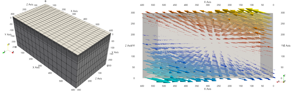
Example: strike-slip model, rotated velocity field and mesh refinement
This example will build a 3D model with vertical
mesh refinement
and a strike-slip velocity field
rotated
by 15 degrees as showed in the figure below.
In addition, 2 gaussian weak zones are added to the initial conditions of the model
1. Create a domain
We define a 3D Domain \(\Omega = [0,600]\times[-250,0]\times[0,300]\) km3
\(\in \mathbb R^3\) discretized by a regular grid of 9x9x9 nodes.
import os
import numpy as np
import genepy as gp

# 3D domain
dimensions = 3
O = np.array([0,-250e3,0],    dtype=np.float64) # Origin
L = np.array([600e3,0,300e3], dtype=np.float64) # Length
n = np.array([9,9,9],         dtype=np.int32)   # Number of Q1 nodes i.e. elements + 1
# Create Domain class instance
Domain = gp.Domain(dimensions,O,L,n)
2. Mesh refinement
In this step we refine the mesh
in the vertical direction (\(y\)) using linear interpolation.
Note however that the mesh refinement can be done in any direction following the same pattern.
# Define refinement parameters in a dictionary
refinement = {"y": # direction of refinement
                  {"x_initial": np.array([-250,-180,-87.5,0], dtype=np.float64)*1e3, # xp
                   "x_refined": np.array([-250,-50,-16.25,0], dtype=np.float64)*1e3} # f(xp)
             }
# Create MeshRefinement class instance
MshRef = gp.MeshRefinement(Domain,refinement)
3. Rotation
To rotate the velocity field we first need to
set the parameters of this rotation.
In this example we perform a rotation of 15 degrees
clockwise around the \(y\) axis.
# Rotation of the referential
r_angle = np.deg2rad(-15.0)                   # Rotation angle \in [-pi, pi]
axis    = np.array([0,1,0], dtype=np.float64) # Rotation axis
# Create instance of Rotation class
Rotation = gp.Rotation(dimensions,r_angle,axis)
4. Velocity field
Next, we create a strike-slip velocity field with a norm of 1 cm.a-1.
The method
evaluate_velocity_and_gradient_symbolic()
returns the symbolic expression of the velocity field and its gradient.
The method
evaluate_velocity_numeric()
returns the numeric value of the velocity field evaluated at coordinates of the nodes.
The method
get_velocity_orientation()
returns the orientation of the velocity field at the boundary.
Note
The rotation of the velocity field is handled inside the velocity function evaluation and does not require any additional step.
# velocity function parameters
cma2ms  = 1e-2 / (3600.0 * 24.0 * 365.0) # cm/a to m/s conversion
u_norm  = 1.0 * cma2ms                   # horizontal velocity norm
u_angle = np.deg2rad(90.0)               # velocity angle \in [-pi/2, pi/2]
u_dir   = "z"                            # direction in which velocity varies
u_type  = "extension"                    # extension or compression, defines the sign
# Create velocity class instance
BCs = gp.VelocityLinear(Domain,u_norm,u_dir,u_type,u_angle,Rotation)

# Access the symbolic velocity function, its gradient and the orientation of the horizontal velocity at the boundary
u      = BCs.u                # velocity function
grad_u = BCs.grad_u           # gradient of the velocity function
uL     = BCs.u_dir_horizontal # orientation of the horizontal velocity at the boundary (normalized)
5. Define gaussian weak zones
In this example we define two gaussian weak zones.
We provide the parameters of the gaussians and their position in the domain.
Note
In this example we rotate the velocity field by 15 degrees.
Therefore we also rotate the gaussians by 15 degrees.
This is achieved by passing the
Rotation class instance to the
Gaussian2D class constructor.
# gaussian initial strain
ng = np.int32(2) # number of gaussians
A  = np.array([1.0, 1.0],dtype=np.float64)
# shape of the gaussians
coeff = 0.5 * 6.0e-5**2
a = np.array([coeff, coeff], dtype=np.float64)
b = np.array([coeff, coeff], dtype=np.float64)
# position of the centre of the gaussians
dz    = 27.5e3                         # distance from the domain centre in z direction
angle = np.deg2rad(75)                 # angle between the x-axis and the line that passes through the centre of the domain and the centre of the gaussian
domain_centre = 0.5*(Domain.O + Domain.L) # centre of the domain

x0 = np.zeros(shape=(ng), dtype=np.float64)
# centre of the gaussian in z direction
z0 = np.array([domain_centre[2] - dz,
               domain_centre[2] + dz], dtype=np.float64)
# centre of the gaussian in x direction
x0[0] = gp.utils.x_centre_from_angle(z0[0],angle,(domain_centre[0],domain_centre[2]))
x0[1] = gp.utils.x_centre_from_angle(z0[1],angle,(domain_centre[0],domain_centre[2]))
# Create gaussian object
G = []
for i in range(ng):
  G.append(gp.Gaussian2D(Domain,A[i],a[i],b[i],x0[i],z0[i],Rotation))
  # print the expression and parameters
  print(G[i])

Gaussian = gp.GaussiansOptions(G)
6. Initial conditions
Gather the information defined previously to generate the options for the initial conditions.
# Initial plastic strain
IniStrain = gp.InitialPlasticStrain(Gaussian)
# Initial conditions
model_ics = gp.InitialConditions(Domain,u,mesh_refinement=MshRef,initial_strain=IniStrain)
7. Boundary conditions
Gather the velocity field information and indicate the type of boundary conditions required to generate the options for the boundary conditions.
Details on the methods used to define the boundary conditions can be found in the boundary conditions section.
# path to mesh files (system dependent, change accordingly)
root = os.path.join(os.environ['PTATIN'],"ptatin-gene/src/models/gene3d/examples")
# Velocity boundary conditions
u_bcs = [
  gp.Dirichlet(tag=23,name="Zmax",components=["x","z"],velocity=u,mesh_file=os.path.join(root,"box_ptatin_facet_23_mesh.bin")),
  gp.Dirichlet(37,"Zmin",["x","z"],u,mesh_file=os.path.join(root,"box_ptatin_facet_37_mesh.bin")),
  gp.NavierSlip(tag=32,name="Xmax",grad_u=grad_u,u_orientation=uL,mesh_file=os.path.join(root,"box_ptatin_facet_32_mesh.bin")),
  gp.NavierSlip(14,"Xmin",grad_u,uL,mesh_file=os.path.join(root,"box_ptatin_facet_14_mesh.bin")),
  gp.DirichletUdotN(33,"Bottom",mesh_file=os.path.join(root,"box_ptatin_facet_33_mesh.bin")),
]
# Temperature boundary conditions
Tbcs = gp.TemperatureBC({"ymax":0.0, "ymin":1450.0})
# collect all boundary conditions
model_bcs = gp.ModelBCs(u_bcs,Tbcs)
8. Material parameters
Next we define the material properties (mechanical and thermal) of the different
regions of the model.
For each region, a set of parameters is defined using the corresponding classes.
The details on the methods can be found in the
material parameters section.
Flow laws parameters can be found in genepy/material_params/arrhenius_flow_laws.json.
# Define the material parameters for the model as a list of Region objects
regions = [
  # Upper crust
  gp.Region(38,                                          # region tag
            gp.DensityBoussinesq(2700.0,3.0e-5,1.0e-11), # density
            gp.ViscosityArrhenius2("Quartzite"),         # viscosity  (values from the database using rock name)
            gp.SofteningLinear(0.0,0.5),                 # softening
            gp.PlasticDruckerPrager(),                   # plasticity (default values, can be modified using the corresponding parameters)
            gp.Energy(heat_source=gp.EnergySource(gp.EnergySourceConstant(1.5e-6),
                                                  gp.EnergySourceShearHeating()),
                      conductivity=2.7)),
  # Lower crust
  gp.Region(39,
            gp.DensityBoussinesq(density=2850.0,thermal_expansion=3.0e-5,compressibility=1.0e-11),
            gp.ViscosityArrhenius2("Anorthite",Vmol=38.0e-6),
            gp.SofteningLinear(strain_min=0.0,strain_max=0.5),
            gp.PlasticDruckerPrager(),
            gp.Energy(heat_source=gp.EnergySource(gp.EnergySourceConstant(0.5e-6),
                                                  gp.EnergySourceShearHeating()),
                      conductivity=2.85)),
  # Lithosphere mantle
  gp.Region(40,
            gp.DensityBoussinesq(3300.0,3.0e-5,1.0e-11),
            gp.ViscosityArrhenius2("Peridotite(dry)",Vmol=8.0e-6),
            gp.SofteningLinear(0.0,0.5),
            gp.PlasticDruckerPrager(),
            gp.Energy(heat_source=gp.EnergySource(gp.EnergySourceShearHeating()),
                      conductivity=3.3)),
  # Asthenosphere
  gp.Region(41,
            gp.DensityBoussinesq(3300.0,3.0e-5,1.0e-11),
            gp.ViscosityArrhenius2("Peridotite(dry)",Vmol=8.0e-6),
            gp.SofteningLinear(0.0,0.5),
            gp.PlasticDruckerPrager(),
            gp.Energy(heat_source=gp.EnergySource(gp.EnergySourceShearHeating()),
                      conductivity=3.3))
]

# path to mesh files (system dependent, change accordingly)
root = os.path.join(os.environ['PTATIN'],"ptatin-gene/src/models/gene3d/examples")
model_regions = gp.ModelRegions(regions,
                                mesh_file=os.path.join(root,"box_ptatin_md.bin"),
                                region_file=os.path.join(root,"box_ptatin_region_cell.bin"))
9. Add surface processes
In this example we add surface processes.
Surface processes are done by solving a diffusion equation.
Here we set "zmin" and "zmax" as Dirichlet boundary conditions for the diffusion equation
and we set the diffusivity to \(10^6\) m2.s-1.
# Add erosion-sedimentation with diffusion
spm = gp.SPMDiffusion(["zmin","zmax"],diffusivity=1.0e-6)
10. Add passive tracers
Add passive tracers to the model. Here we define a box \(x \in [0, 600] \times y \in [-100, 0] \times z \in [0, 300]\) km3 of passive tracers with a layout of \(30 \times 5 \times 15\) lagrangian markers. We activate the tracking of the pressure and temperature fields.
Note
Other types of passive tracers layout can be found in the
passive tracers section.
# Add passive tracers
pswarm = gp.PswarmFillBox([0.0,-100.0e3,0.0],
                          [600e3,-4.0e3,300.0e3],
                          layout=[30,5,15],
                          pressure=True,
                          temperature=True)
11. Create the model and generate options
The model is created by gathering all the information defined previously.
# write the options for ptatin3d
model = gp.Model(model_ics,model_regions,model_bcs,
                 model_name="model_GENE3D",
                 spm=spm,pswarm=pswarm)
with open("strike-slip.opts","w") as f:
  f.write(model.options)