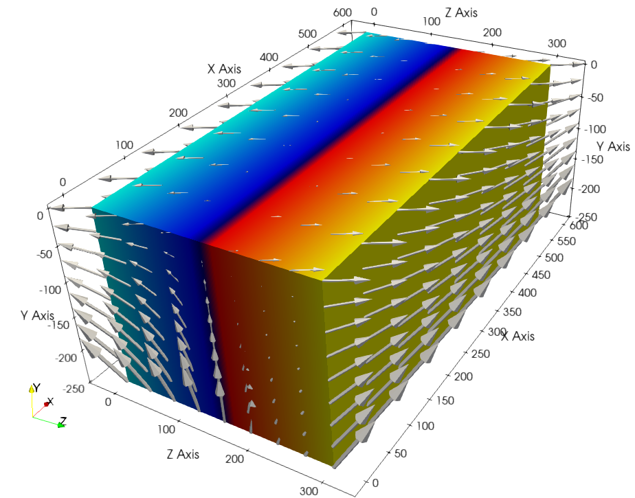
Example: oblique model, non-linear rheology
In this example we build a model with an oblique velocity field to impose
extension at 30 degrees (counter-clockwise) with respect to the \(z\) axis
(can be seen as north-south direction).
We use non-linear viscous rheology,
Drucker-Prager plasticity and
a combination of Dirichlet and
Navier-slip type boundary conditions.
1. Create a domain
We define a 3D domain \(\Omega = [0,600]\times[-250,0]\times[0,300]\) km3 \(\in \mathbb R^3\) discretized by a regular grid of 9x9x9 nodes.
import os
import numpy as np
import genepy as gp

# 3D domain
dimensions = 3
O = np.array([0,-250e3,0],    dtype=np.float64) # Origin
L = np.array([600e3,0,300e3], dtype=np.float64) # Length
n = np.array([9,9,9],         dtype=np.int32)   # Number of Q1 nodes i.e. elements + 1
# Create Domain class instance
Domain = gp.Domain(dimensions,O,L,n)
2. Velocity function
We define an oblique extension velocity velocity field
forming an angle of 30 degrees counter-clockwise with respect to the \(z\) axis.
The VelocityLinear class attributes
uis the symbolic velocity functiongrad_uis the symbolic gradient of the velocity functionu_dir_horizontalis the orientation of the horizontal velocity at the boundary
# velocity
cma2ms  = 1e-2 / (3600.0 * 24.0 * 365.0) # cm/a to m/s conversion
u_norm  = 1.0 * cma2ms                   # horizontal velocity norm
u_angle = np.deg2rad(30.0)               # velocity angle \in [-pi/2, pi/2]
u_dir   = "z"                            # direction in which velocity varies
u_type  = "extension"                    # extension or compression
# Create Velocity class instance
BCs = gp.VelocityLinear(Domain,u_norm,u_dir,u_type,u_angle)

# Access the symbolic velocity function, its gradient and the orientation of the horizontal velocity at the boundary
u      = BCs.u                # velocity function
grad_u = BCs.grad_u           # gradient of the velocity function
uL     = BCs.u_dir_horizontal # orientation of the horizontal velocity at the boundary (normalized)
3. Initial conditions
In this example we do not impose any initial plastic strain value nor mesh refinement.
Therefore the initial conditions
are only the Domain and the velocity function.
They will be used to generate the options for pTatin3d model.
# Initial conditions
model_ics = gp.InitialConditions(Domain,u)
4. Boundary conditions
Because the imposed velocity is oblique to the boundary we define the
velocity boundary conditions using Dirichlet and
Navier-slip type boundary conditions.
Note that the Dirichlet conditions takes now the 2 horizontal components to impose the obliquity.
Moreover, we will use non-linear viscosities depending of the temperature so we need to provide boundary conditions for the conservation of the thermal energy.
Details on the methods used to define the boundary conditions can be found in the boundary conditions section.
# boundary conditions
# path to mesh files (system dependent, change accordingly)
root = os.path.join(os.environ['PTATIN'],"ptatin-gene/src/models/gene3d/examples")
# Velocity boundary conditions
u_bcs = [
  gp.Dirichlet( 23,"Zmax",["x","z"],u, mesh_file=os.path.join(root,"box_ptatin_facet_23_mesh.bin")),
  gp.Dirichlet( 37,"Zmin",["x","z"],u, mesh_file=os.path.join(root,"box_ptatin_facet_37_mesh.bin")),
  gp.NavierSlip(32,"Xmax",grad_u,uL,   mesh_file=os.path.join(root,"box_ptatin_facet_32_mesh.bin")),
  gp.NavierSlip(14,"Xmin",grad_u,uL,   mesh_file=os.path.join(root,"box_ptatin_facet_14_mesh.bin")),
  gp.DirichletUdotN(33,"Bottom",       mesh_file=os.path.join(root,"box_ptatin_facet_33_mesh.bin")),
]
# Temperature boundary conditions
Tbcs = gp.TemperatureBC({"ymax":0.0, "ymin":1450.0})
# collect all boundary conditions
model_bcs = gp.ModelBCs(u_bcs,Tbcs)
5. Material parameters
Next we define the material properties of each Region and
gather them all in a ModelRegions class instance.
In this example we use the following material types:
Drucker-Pragerplastic yield criterion.
Flow laws parameters can be found in genepy/material_params/arrhenius_flow_laws.json.
regions = [
  # Upper crust
  gp.Region(38,                                          # region tag
            gp.DensityBoussinesq(2700.0,3.0e-5,1.0e-11), # density
            gp.ViscosityArrhenius2("Quartzite"),         # viscosity  (values from the database using rock name)
            gp.SofteningLinear(0.0,0.5),                 # softening
            gp.PlasticDruckerPrager(),                   # plasticity (default values, can be modified using the corresponding parameters)
            gp.Energy(heat_source=gp.EnergySource(gp.EnergySourceConstant(1.5e-6), # energy
                                                  gp.EnergySourceShearHeating()),
                      conductivity=2.7)),
  # Lower crust
  gp.Region(39,
            gp.DensityBoussinesq(density=2850.0,thermal_expansion=3.0e-5,compressibility=1.0e-11),
            gp.ViscosityArrhenius2("Anorthite",Vmol=38.0e-6),
            gp.SofteningLinear(strain_min=0.0,strain_max=0.5),
            gp.PlasticDruckerPrager(),
            gp.Energy(heat_source=gp.EnergySource(gp.EnergySourceConstant(0.5e-6), # energy
                                                  gp.EnergySourceShearHeating()),
                      conductivity=2.85)),
  # Lithosphere mantle
  gp.Region(40,
            gp.DensityBoussinesq(3300.0,3.0e-5,1.0e-11),
            gp.ViscosityArrhenius2("Peridotite(dry)",Vmol=8.0e-6),
            gp.SofteningLinear(0.0,0.5),
            gp.PlasticDruckerPrager(),
            gp.Energy(heat_source=gp.EnergySource(gp.EnergySourceShearHeating()),
                      conductivity=3.3)),
  # Asthenosphere
  gp.Region(41,
            gp.DensityBoussinesq(3300.0,3.0e-5,1.0e-11),
            gp.ViscosityArrhenius2("Peridotite(dry)",Vmol=8.0e-6),
            gp.SofteningLinear(0.0,0.5),
            gp.PlasticDruckerPrager(),
            gp.Energy(heat_source=gp.EnergySource(gp.EnergySourceShearHeating()),
                      conductivity=3.3))
]
model_regions = gp.ModelRegions(regions,
                                mesh_file=os.path.join(root,"box_ptatin_md.bin"),
                                region_file=os.path.join(root,"box_ptatin_region_cell.bin"))
6. Create the model and generate options
Finally, we create the model by gathering all the information defined previously and we save
the options to a file named oblique_extension_model.opts.
# create class instance
model = gp.Model(model_ics,model_regions,model_bcs)
# write the options for ptatin3d
with open("oblique_extension_model.opts","w") as f:
  f.write(model.options)