Building a mesh with Gmsh for the initial geometry and boundary conditions
pTatin3d represents the materials on lagrangian markers populating the domain. The markers are attributed a “phase” index which is used to assign the material properties. To generalise the creation of models with pTatin3d we rely on Gmsh to create a mesh that will hold the initial geometry of the model and the physical position of the boundary conditions.
Note
The mesh created with Gmsh is not used to solve the problem, pTatin3d creates its own structured mesh. It is only used to create the initial geometry and identify boundaries. Therefore, the mesh should be as coarse as possible to fasten its creation, ease its portability between machines and fasten the location of the lagrangian markers from pTatin3d inside this mesh.
Note
It is strongly recommended for beginners to use the Gmsh GUI to build the mesh. A nice feature of Gmsh GUI is that you can edit the .geo file dynamically while performing operations in the GUI. This is a good way to learn the syntax of the .geo file and understand how Gmsh works.
Warning
When using a free-surface boundary condition for the surface of the domain, the mesh will deform. However, we use the Gmsh surfaces to define the boundary conditions in pTatin3d. Therefore, if the pTatin3d mesh falls outside the Gmsh mesh, the boundary conditions will not be applied. To prevent this, it is required to create a mesh with Gmsh taking in account that the surface in pTatin3d may uplift. To do so you can set the \(y\) coordinate of the points defining the surface in Gmsh to an altitude that will never be reached in the geodynamic simulation.
1. Points
The first step is to create the points that will define the geometry of the model. Two possibilities are available to create points in Gmsh:
directly in the graphical interface with the Geometry \(\rightarrow\) Elementary entities \(\rightarrow\) Add \(\rightarrow\) Point
by editing the .geo file using the following syntax:
Point(1) = {0, 0, 0, lc};
Point(2) = {1, 0, 0, lc};
Point(3) = {1, 1, 0, lc};
Point(4) = {0, 1, 0, lc};
whith the syntax
Point(i) = {x, y, z, lc};whereiis the index of the point,x,yandzare the coordinates of the point andlcis the size of the mesh around the point.
Note
Editing the .geo file is more efficient when creating a large number of points because it can be generated using a script.
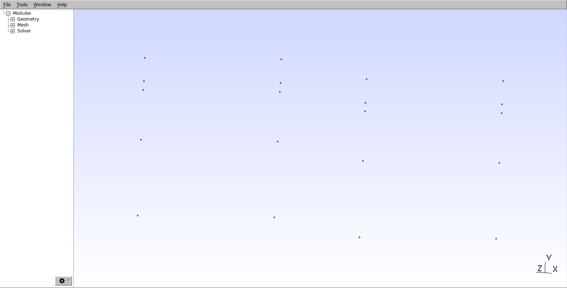
In the Gmsh GUI you will obtain points as shown in the figure below:
2. Lines
The next step is to connect points to create lines. Lines should connect points to create closed loops that will next be utilised to define the surfaces of the model. Lines should not cross each other. If they cross, prefer creating a point at the intersection and connect the lines to this point.
Just like for points, lines can be created in the GUI or by editing the .geo file.
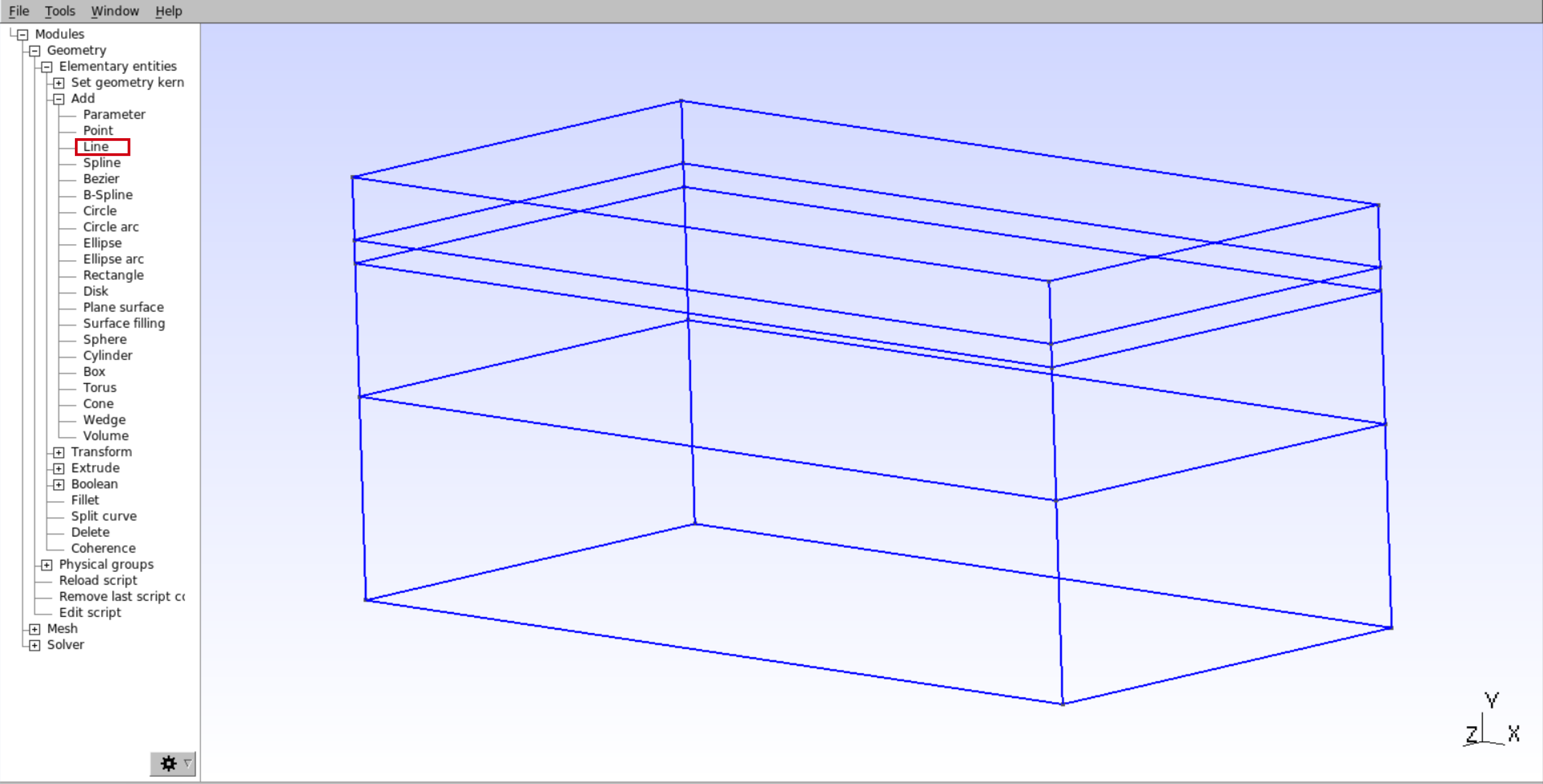
In the GUI use Geometry \(\rightarrow\) Elementary entities \(\rightarrow\) Add \(\rightarrow\) Line.
In the .geo file use Line(i) = {p1, p2}; where i is the index of the line and p1 and p2 are the indices of the points.
You will obtain lines as shown in the figure below:
3. Surfaces
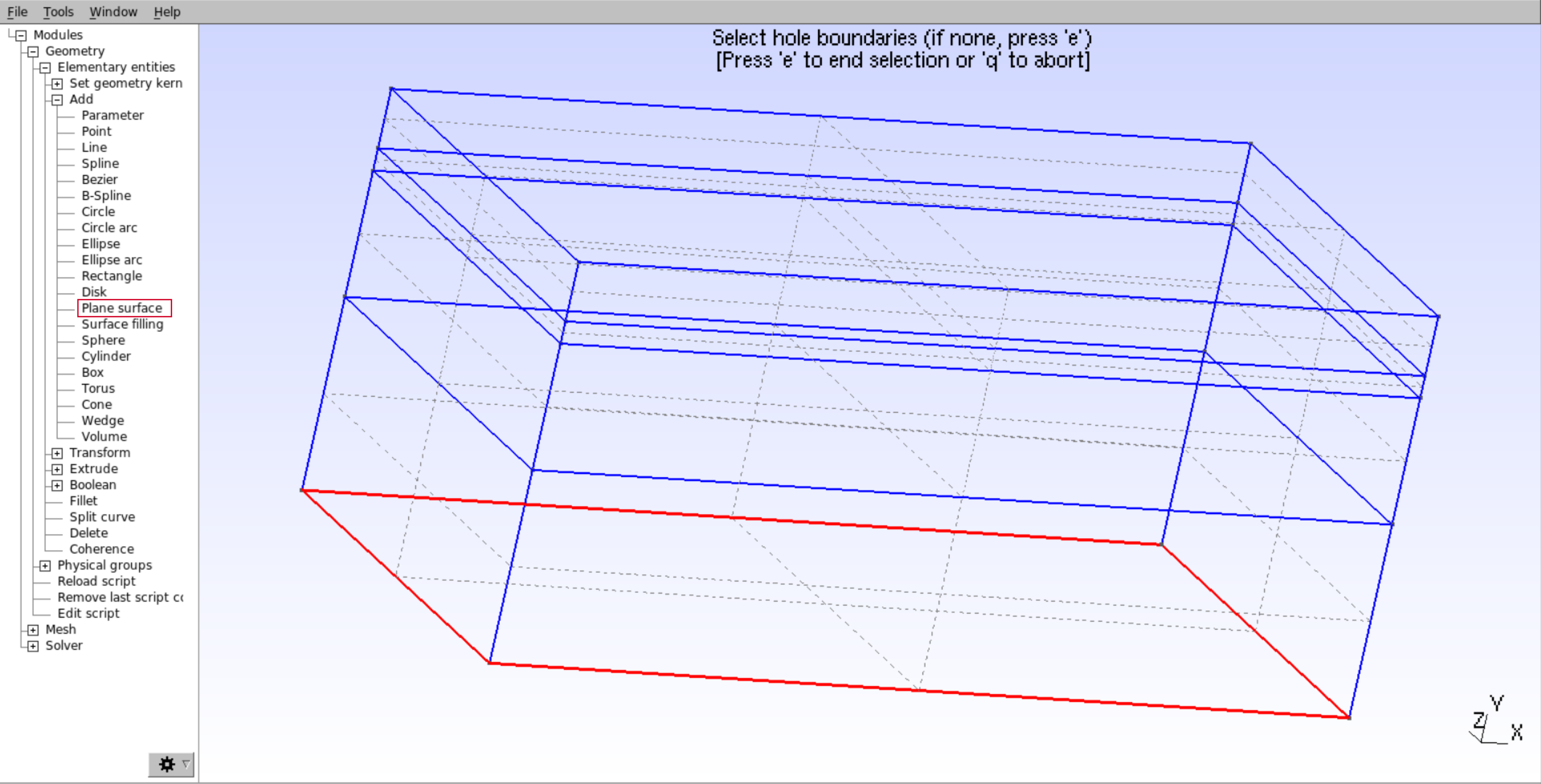
Once points closing a surface have been connected by lines the next step is to create the surfaces. Surfaces can be created using the GUI with Geometry \(\rightarrow\) Elementary entities \(\rightarrow\) Add \(\rightarrow\) Plane surface. This tool will ask you to select the lines that close the surface:
You need to repeat this operation for each surface of the model (both internal and external surfaces). Again you can use the .geo file to create the surfaces. However, at this point the organization of the .geo file starts to be more complex and keeping track of the indices of the lines that close the surfaces can be difficult.
4. Volumes
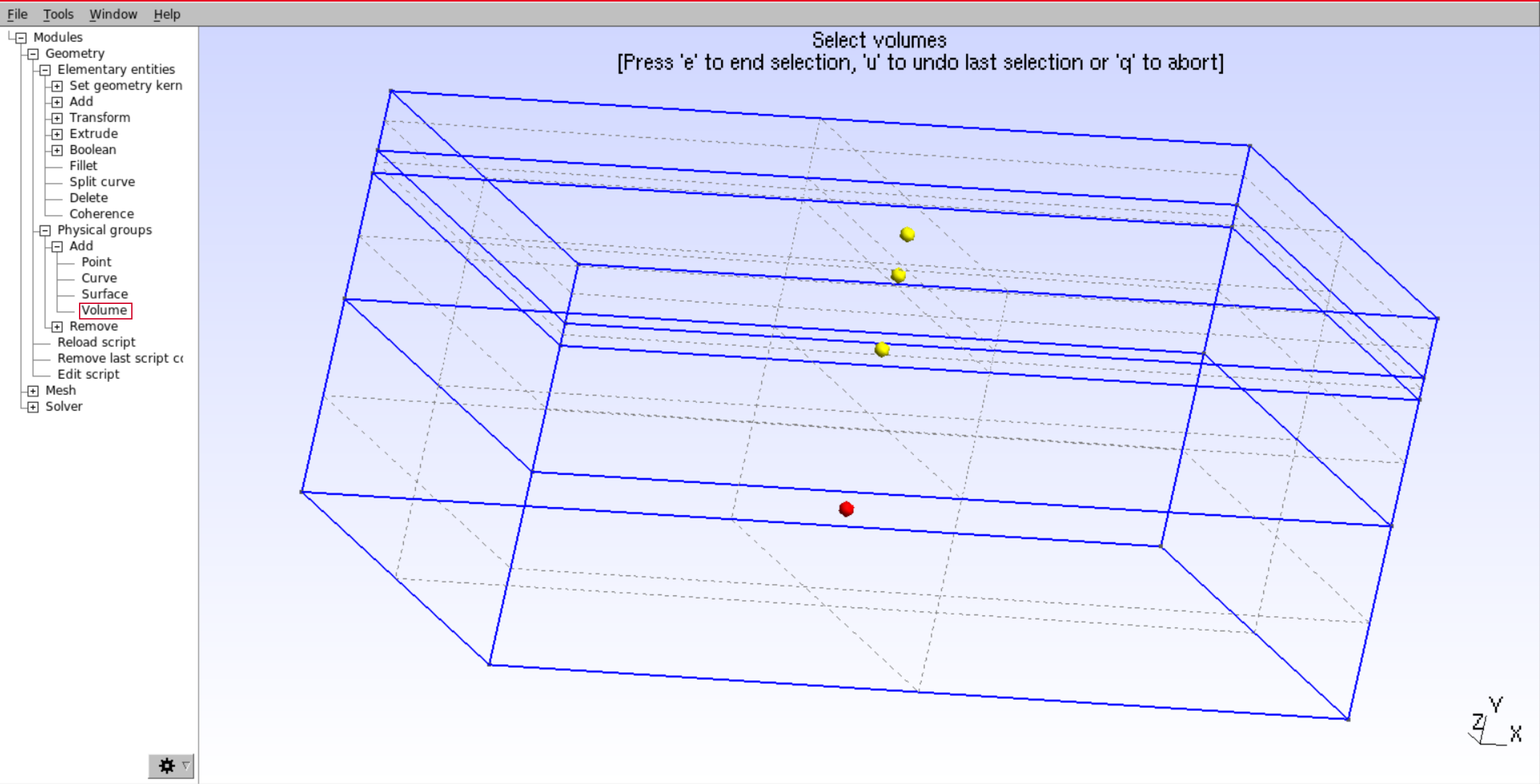
Once the surfaces have been created, the next step is to create the volumes. Like surfaces, volumes are built by selecting the surfaces that close the volume. This can be done in the GUI with Geometry \(\rightarrow\) Elementary entities \(\rightarrow\) Add \(\rightarrow\) Volume.
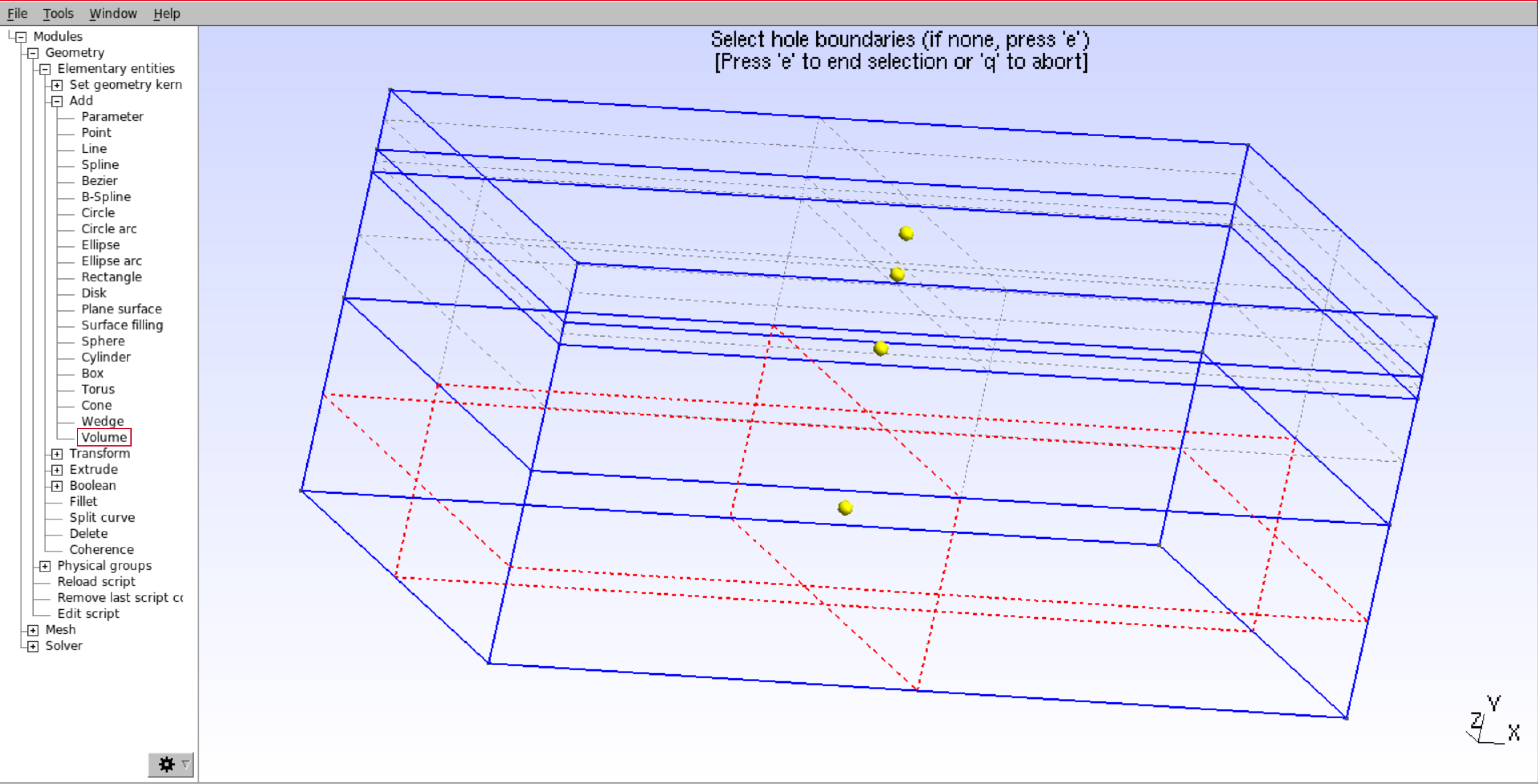
You need to repeat this operation for each volume of the model.
5. Physical groups
Once the surfaces and volumes of the model have been created the next step is to define the physical groups. Physical groups are used for two purposes: 1. To define the materials of the model. 2. To define the boundary conditions of the model.
When creating a physical group, Gmsh assigns a tag to the group. pTatin3d uses this tag to identify the group and assign the correct material properties or boundary conditions.
Warning
pTatin3d cannot handle tags greater than 700. Please use tags smaller than 700.
To create a physical group in Gmsh with the GUI use Geometry \(\rightarrow\) Physical groups \(\rightarrow\) Add \(\rightarrow\) Surface for surfaces or Geometry \(\rightarrow\) Physical groups \(\rightarrow\) Add \(\rightarrow\) Volume for volumes.
These will ask you to select either volumes or surfaces you want to group as the same physical group. It means that you can group several surfaces or volumes in the same physical group. As an exemple, if you have two volumes separated in space but made of the same material, you can group them in the same physical group. The same applies for boundary conditions, if you have two boundaries that have the same boundary condition, you can group them in the same physical group.
Note
You can choose the tag you want to apply to the physical group. You can also choose the name of the physical group which helps to identify the group in the .geo file. The .geo file will record the physical groups with the following syntax:
Physical Volume("upper_crust", 38) = {1};
Physical Surface("zmax", 37) = {14, 15, 16, 17};
In this exemple, "upper_cruts" is the name of the volume physical group, 38 its tag and {1}
the volumes that are in this group and
"zmax" is the name of the surface physical group, 37 its tag and {14, 15, 16, 17}
the surfaces that are in this group.
6. Mesh
Finally, once everything is set up, the last step is to create the mesh. In the GUI use Mesh \(\rightarrow\) 3D to create the mesh.

Once it is done you can save the mesh using File \(\rightarrow\) Save mesh.
Again, this mesh is not utilised to solve any PDE. Therefore, try to create it the coarsest possible.
7. Export The last step is to export the mesh from the .msh format to files that pTatin3d will interpret to create the model. This step requires you to download and install the python package gmsh_to_point_cloud. Follow the installation instructions on the github page of the package. Once it is installed move to the branch of the package that is compatible with pTatin3d:
git checkout anthony_jourdon/surface-tag
Then you can generate the files for pTatin3d with:
python parse_regions_from_gmsh.py -f your_mesh.msh
This will generate a set of files named:
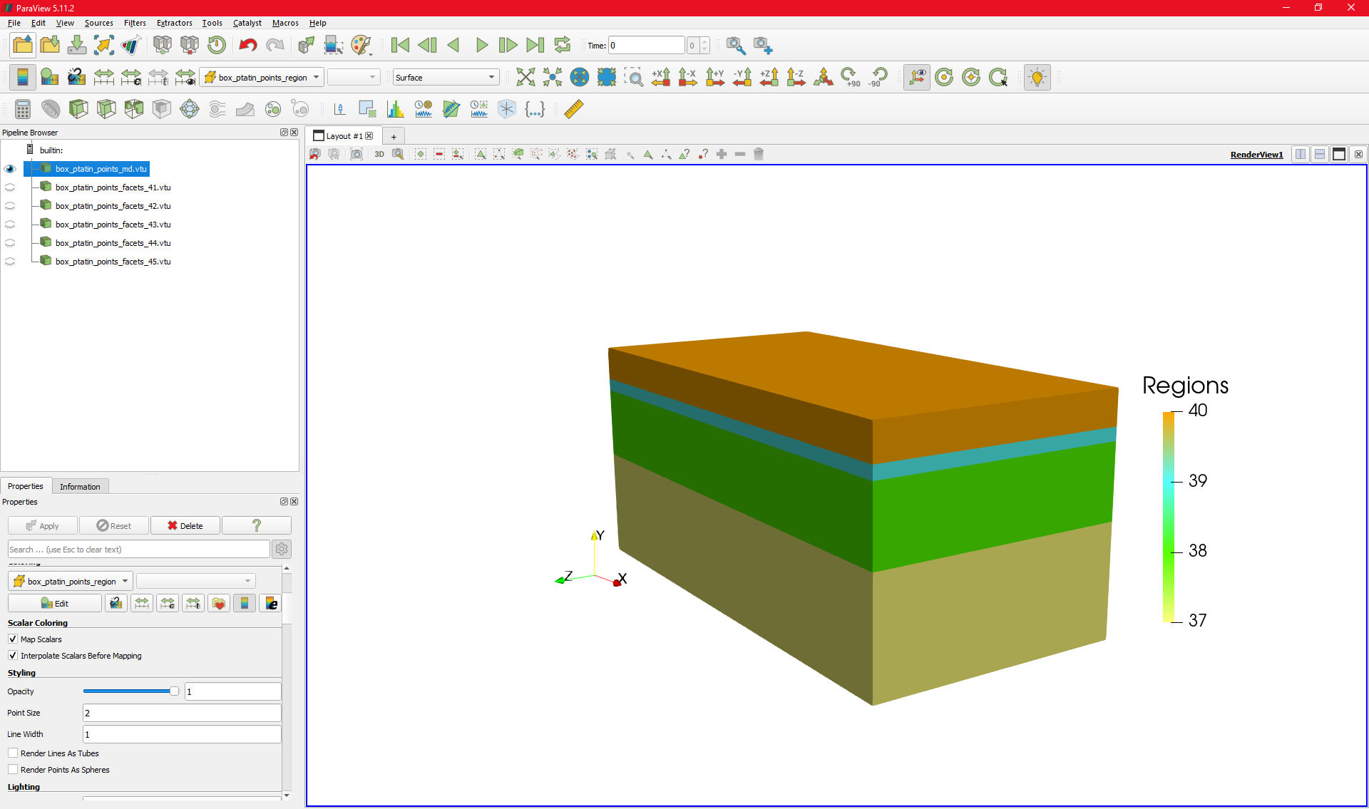
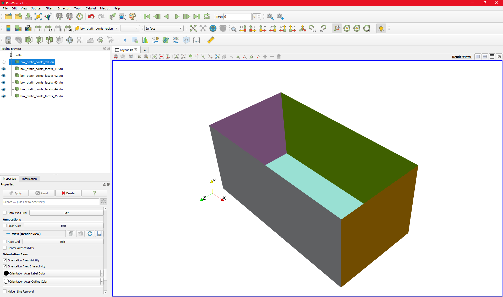
*_md.bincontaining the mesh (element-to-vertex connectivity and vertices coordinates)*_region_cell.bincontaining the region of each cell*_md.vtucombining the mesh and region cell in a .vtu file that can be visualised with Paraview to verify that it is what you expect.*_facet_*_mesh.bincontaining the mesh of the facets of the model with its tag used for boundary conditions.*_facets_*.vtuwhich is the same than the .bin file but in .vtu format to visualise the facets with Paraview.
Note
Only the .bin files are used by pTatin3d. The .vtu files are only for visualisation purposes.
As an example, here are the files generated for a simple model with 4 flat layers, a free-surface and 5 boundaries:
Warning
Any portion of a boundary that is not tagged into a physical surface will be considered as a free-surface:
Therefore, the top surface does not need to be tagged, however, if the gravity acceleration is non-zero, using a free-surface boundary condition on any other face than the top face will lead to an outflow of material under the effect of gravity.